Data Architecture

GitHub - arpit-mittal-ds/Data-Architect-Udacity-Nanodegree: plan, design and implement enterprise data infrastructure solutions and create the blueprints for an organization’s data management system. You’ll create a relational database with PostGreSQL, design an Online Analytical Processing (OLAP) data model to build a cloud based data warehouse, and design scalable data lake architecture that meets the needs of Big Data. Finally, you’ll learn how to apply the principles of data governance to an organization’s data management system.GitHub

help.com is for sale | www.oxley.com

OLTP vs. OLAP

Think about how fast you want the data to be refreshed. If you need data to be refreshed rapidly and frequently, that is OLTP or transactional. If you don't need the data to be refreshed frequently, that's OLAP or reporting. https://www.guru99.com/oltp-vs-olap.html

Data ModelingAnalytics4All

What is a Database SchemaLucidchart

More importantly, we learned how to do normalize data, taking a data set, and working through the steps of the 1st, 2nd, and finally 3rd Normal Forms. It may seem tricky at first, but do it a few times, and normalizing data becomes almost second nature.

1NF rules

• Uses entities (tables)

• Each cell in an attribute (column) has an atomic value (a single value)

• No repeated groupings

• No duplicate rows

2NF rules

• Everything from 1NF

• Ensure data integrity

• All columns depend on the unique ID

3NF rules

• Everything from 2NF

• Remove transitive dependencies

Note about statistical normalization

Anyone familiar with basic statistics may have seen the term normalization before. In statistics, normalization means utilizing mathematical techniques to change the distribution of the data set to more resemble a normal bell curve. This is not what we are talking about in this course. Normalization in the context of data modeling is about reorganizing data for better writing speed and data integrity preservation. While the naming conventions are similar the two topics are not related and should not be confused.

To normalize data to 3NF, follow these steps

1. Check if tables are in 1NF

   Tables should have atomic value, no repeated groupings, and no repeated rows. If any of the 1NF rules is not met, you are not in 1NF. You can create new entities to solve the problem.

2. Develop a data hierarchy

   Hierarchy can help you determine how many entities to start with and how they relate. Based on the hierarchy, you can group data into different entities with attributes.

3. Make sure all the entities are still in 1NF and also follow 2NF rules

   2NF requires that no duplicates and every column depends on the unique ID. In most cases, you can add unique IDs and create new entities to meet the 2NF requirements.

4. Transform the entities from 2NF to 3NF

   You can complete this by checking if there are any transitive dependencies. If there is, you should create another entity to hold the transitive column.

Build Conceptual ERDs

Keep in mind, conceptual ERDs are often a first pass, and the relationships between entities not fully defined. It's common to have to return to your conceptual model to adjust relationships as the model is more fully fleshed out.

Remember, the conceptual model simply has the entities and lines indicating their relationship paths.

You can follow these steps to build conceptual ERDs:

• Determine the type of database to be designed

• Evaluate data (if provided)

• Put data into 3NF

• Place entities on the diagram

• Connect entities with a relationship line

Conceptual ERD example

Below are some great articles on ERD design and development. The sign visual-paradigm is a great resource for information on ERDs.

• This article on introduction to ERDs is from LucidChart, the software tool we are using in this course.

• The site visual-paradigm is a great resource for information on ERDs. article 1 and article 2

Build Conceptual And Logical ERD Walkthrough

The main take away from this exercise is the mapping entity that maps out the complex relations between drivers, limos, and jobs. Remember, when you encounter a complex relationship, you may consider using a mapping entity as a pivotal table to straighten it.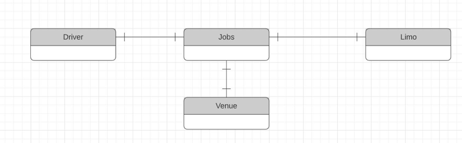

Conceptual ERD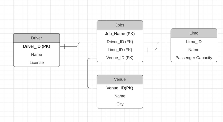

Crow’s Foot Notation

Crow’s Foot Notation

példa: ERD

There is a player history table to store the start and end data.

Conceptual ERD

Logical ERD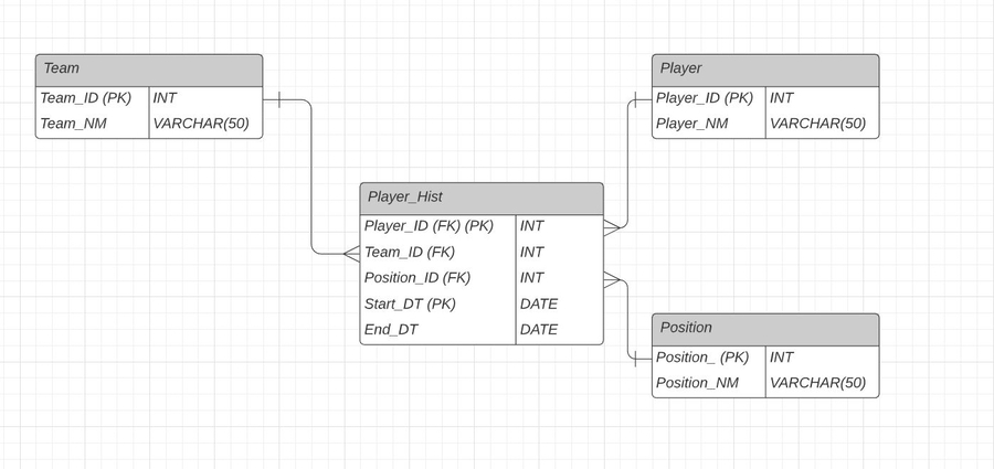

Physical ERD

Note: here I added the PK to the Player_Hist table. It is a combined PK which consists of more than one attribute (Start_DT and Player_ID).

Second Solution

There is no Player history table. Instead, date info is stored in the Player table. It requires a complex primary key and does not provide much flexibility for future table additions.

Here we focus on database performance. There are many factors that can harm database performance:

• Massive amounts of data

• Complex joins

• Complex queries

• Insufficient hardware

• Poor network performance

While many of the aspects affecting database performance are generally out of the hands of data architect, we focused on two common aspects you should be aware of: Cache and Indexing. Both can improve database performance, and you should be aware of the uses of both technologies.

Cache

Cache is a place to store commonly used data in high-performance memory so the future queries for that data can be run faster.

There are three types of cache:

• Internal cache: internal device, limited size, fastest memory, very expensive financially.

• External cache: external device, high-speed memory, upgrading the size of memory is more affordable than internal cache.

• Enterprise cache: external device, designed to work for multiple databases, very expensive.

Indexing

Indexing is creating a lookup table for a database table. It is specifically tuned to search for specific information in a table.

Three types of cache

Further reading

For further reading on cache, I am including the link to an AWS whitepaper on their standard database caching strategies.

This link is a great article on database indexing, It has some great graphics that really help clear up the concept of database indexing.

Storage algorithm

It is purely academic. As a data architect, you will not be developing or designing data storage algorithms, but knowing the basics of the most common data storage approaches may come in handy in the interview one day.

• Heap files: Heap files are a group of unordered lists of records where new records are appended to the end of the existing lists. This algorithm allows very fast writing and is perfect for the bulk loading of data. But it has poor sorting performance since the data is not ordered, which makes retrieving specific data very slow.

• Hash buckets: Buckets divide memory into pages and when a record comes in, a hash function (math function) is calculated to determine which page it goes on. This algorithm ensures more even distribution of records across the memory. It is good for locating specific records since it creates a kind of key index. But it is not good for large data retrieval, since it has no sequential storage (meaning records are not stored in order, one after the other, they are instead stored across multiple pages based on their hash value).

• B+ trees: B+ tree is the most commonly used storage algorithm. It stores records in pages as well, but it indexes the record in a binary tree. It allows fast search due to the full index and binary design. It can also be easily scaled up for large databases. However, for stable, not volatile data, a heap file may work better since heap has less overhead.

As I mentioned, the first part of this section is purely for academic purposes. However, you want to dive deeper into Heap Files and B+ Trees, here are some good resources:

• Heap Files: Reading 1 and Reading 2

• Hash Buckets: Reading 1 and Reading 2

• B+ Trees: Reading 1 and Reading 2

Use DDL to Create A Database

Data Definition Language - DDL, is a subset of SQL commands used to create, modify and delete database objects. In PostgreSQL, the most commonly used DDL commands are Create, Alter, and Drop.

In the video, we covered the uses of each command, as well as how to add PKs and FKs.

We also introduced a special data type, SERIAL. This is an auto-incrementing integer. Meaning, it starts counting at 1 and continues up for each row you add to a table. Great for creating unique IDs.

Create command

Create table Table_Name(
column_name data type,
column2_name data type);

-- example
Create table Employee(
emp_id int,
emp_NM varchar(50));

-- use SERIAL data type
Create table Employee(
emp_id SERIAL,
emp_nm varchar(50));

Add PK and FK

-- add PK
Create table Employee(
emp_id SERIAL primary key,
emp_NM varchar(50));

-- add FK
Create table Company_Car(
car_id SERIAL primary key,
car_desc varchar(255),
emp_id int REFERENCES Employee(emp_id));

-- add combined PK
Create table Car_Map (
emp_id int REFERENCES Employee(emp_id),
car_id int REFERENCES Company_Car (car_id),
Primary key (emp_id, car_id));

Alter command

-- create a table
Create table Employee(
emp_id int,
emp_NM varchar(50));

-- modify a column
Alter table Employee
Alter column emp_id SERIAL;

-- add a column
Alter table Employee
Add column Address varchar(255);

-- delete a column
Alter table Employee
Drop column Address; 

Drop command

Drop object_type object_name

-- delete a column
Drop column Address

-- delete a table
Drop table Employee 

Here are is an overview article of DDL, DML, and even DCL and TCL (which we do not cover in this course).

Here is the official PostGreSQL documentation on DDL.

4MB

nd038-darch-c1-l4-a08-use-ddl-to-create-a-database-walkthrough_720p.mp4

Using DDL SQL commands, create the database objects depicted in the physical ERD below in the workspace PostgreSQL environment.

CREATE TABLE Player (
player_id SERIAL primary key,
player_nm varchar(50));

CREATE TABLE Team (
team_id  SERIAL primary key,
team_nm varchar(50));

CREATE TABLE Position (
position_id  SERIAL primary key,
position_nm varchar(50));

CREATE TABLE Player_Hist (
player_id int REFERENCES Player(player_id),
team_id int REFERENCES Team(team_id),
position_id int REFERENCES position(position_id),
start_dt date,
end_dt date,
Primary key (player_id, team_id, position_id));

CRUD

CRUD is a common acronym in SQL. It stands for Create, Read, Update, Delete. CRUD is just a name for a series of commands, many of which you already have probably used.

Update and delete fall into the DML category - data manipulation language.

In this section, we just wanted to do a quick SQL refresher, so you can use CRUD commands to demonstrate your database works as promised.

Create

Create object_type object-name 
(parameters);

-- example
Create table Test (
Column_a int,
Column_b varchar(50));

Read

-- select all
Select *
From Test;

-- select column
Select Column_A
From Test;

-- limit result
Select *
From Test
Where Column_B = ‘Hello’

Update

-- insert, add data to a table
Insert into Test (Column_A, Column_B)
Values (1, ‘Hello’),
(2, ‘Good-bye’);

-- update, change existing values in a table
Update Test 
Set Column_B = ‘Bonjour’
Where Column_A = 1;

Delete

-- delete individual records
Delete from Test
Where Column_A = 1;

-- delete everything from the table
Truncate table Test;

Further reading

Below you will find a series of articles on basic SQL functions need to complete this section and your final project. Note, these articles are written for MS SQL Server, but they cover the main topics.

• Select function

• Select functions count, distinct, max, min

• The where clause

• Aggregates group by, having

• Case statements

• Intro to Joins

• 4 types of joins

Data Architecture

Enterprise Data ArchitectureMedium

What artifacts are needed to design a good Data Architecture strategy?

To implement a good Data Architecture strategy, an organization has to create certain documents, known in business as “artifacts”. Following is a list of the major documents to include:

• Data dictionary: helps to standardize business vocabulary

• Enterprise Data models: used to create an ODS (Operational Data Store). We will discuss ODS later in the course

• Data flows: enable a smooth transition of data movements crossing various silos. Later in this video, we will dive deep into data flows

• Data stewardship: specifies who can access what data

• Dimensional models: used to create a data warehouse structure for effective reporting and analytics

• Data sharing agreements: articulate who can access what data

These documents help provide a route map for data flows

Business Artifacts

Alongside the data-related documents above, on the business side, there is also some documentation that is necessary:

• Business rules: guard the boundaries of those data flows.

• Business concepts: help everyone to be on the same page

• Business requirements: help to decide and build reporting and analytics

Why are Artifacts important?

• Capture knowledge so new employees can be trained

• Document the tribal and institutional knowledge of experienced and critical employees, as well as existing employees

• Reduce business risk by documenting the business systems and processes. If some key employees leave the company, without having documentation of their knowledge, it is a big risk to the business.

• Reduce costs by understanding the data and business processes in order to avoid having ineffective and inefficient systems.

• Employee productivity increase with well-defined and understood systems and processes

Getting Started in Snowflake

Creating Schemas in the Snowflake browser

Loading a small file using Snowflake in the browser

Demo Setting up file formats for data loading

Loading data with the Snowflake Client

• Login to your account using the terminal

  • If you need help connecting, you can look back to the Demo: Getting Started in Snowflake in the Data Architecture lesson.

• After successfully entering your password, select the database you can to create this table in (In this demo, we will use the same database we created in the beginning lesson)

  • Use DATABASE xxxxxx;

• Keep using the public schema (but you can change it if you want. )

  • use SCHEMA xxxx;

• Since we will be uploading JSON files we need to create a file format for JSON,

  • create or replace file format myjsonformat type = 'JSON' strip_outer_array=true;

• Using the JSON format we just created, now create a temporary "holding area" for data called a staging file

  • create or replace stage my_json_stage file_format = myjsonformat ;

Creating Tables, Uploading files, and Copying data into the table

• Create a table with one column of type variant.

  • create table userdetails(usersjson variant) ;

• To upload the data from your local computer to the temporary "holding area" stagefile area

  • put file:’your local file location’/filename.json @my_json_stage auto_compress=true;

  • Press enter. If you see uploaded that means the command ran successfully. Note: We compressed the file to speed up the upload.

• Now finally copy the data you just uploaded directly into the table created in the previous steps,

  • copy into userdetails from @my_json_stage/userdetails.json.tz file_format = (format name = myjsonformat on_error = 'skip file';

  • Press If you see the status LOADED it means the data was successfully loaded from the staging area to the table.

Apply Normalization Rules

Transforming JSON data into flat tables Demo for the ODS system

ETL data from staging schema into ODS schema

Login into Snowflake. Review the ERD provided below. This exercise assumes you completed the Staging Area Exercise: Loading small data files where you successfully uploaded the 9 CSV files(Cleaning Testing Exercise Files). For this exercise, you will create relationships in the ODS table with respect to the diagram provided. If needed, those files (called Cleaning_Testing_Files-1) are also located in the resources section of this page.

Create new schema

create schema ODS;

Create complex table and insert

create table complex(complex_id string not null unique, complex_name string, constraint pk_complex_id primary key (complex_id));

now insert the data

insert into complex select * from staging.complex;

Create employee table and insert

create table employee(employee_id number, First_name string, Last_name string, Badge_Status string, Work_from string, constraint pk_employee_id primary key (employee_id)); insert into employee select * from staging.employee;

Create protocol table and insert

create table protocol(protocol_id number, step_id number, step_name string, constraint pk_protocol_id primary key (protocol_id));

now insert the data

insert into protocol select * from staging.protocol;

create hightouchareas table and insert

create table hightouchareas(spot_id number, high_touch_area string, constraint pk_spot_id primary key (spot_id));

now insert the data

insert into HighTouchAreas select * from staging.HighTouchAreas;

create facility table and insert

create table facility(building_id number, building_name string, sqft string, complex_id string, constraint pk_building_id primary key (building_id), constraint fk_complex_id foreign key (complex_id) references complex(complex_id) );

now insert the data

insert into facility select * from staging.facility;

Create floors table and insert

create table floors(floor_id number, floor_name string, building_id number, constraint pk_floor_id primary key (floor_id), constraint fk_building_id foreign key (building_id) references facility(building_id) );

now insert the data

insert into floors select * from staging.floors;

Create rooms table and insert

create table rooms(room_id number, room_name string, floor_id number, building_id number, total_area string, cleaned_area string, constraint pk_room_id primary key (room_id), constraint fk_floor_id foreign key (floor_id) references floors(floor_id), constraint fk_building_id foreign key (building_id) references facility(building_id) );

now insert the data

insert into rooms select * from staging.rooms;

Create frequency table and insert

create table frequency(frequency_id number, building_id number, Frequency number, constraint pk_frequency_id primary key (frequency_id), constraint fk_building_id foreign key (building_id) references facility(building_id) );

now insert the data

insert into frequency select * from staging.frequency;

Create CleaningSchedule table and insert

create table CleaningSchedule(transaction_id number, step_id number, cleaned_on string, frequency_id number, building_id number, floor_id number, room_id number, employee_id number, spot_id number, test_value number, Efficiency number, constraint pk_transaction_id primary key (transaction_id), constraint fk_frequency_id foreign key (frequency_id) references frequency(frequency_id), constraint fk_building_id foreign key (building_id) references facility(building_id), constraint fk_floor_id foreign key (floor_id) references floors(floor_id), constraint fk_room_id foreign key (room_id) references rooms(room_id), constraint fk_employee_id foreign key (employee_id) references employee(employee_id), constraint fk_spot_id foreign key (spot_id) references hightouchareas(spot_id) );

now insert the data

insert into CleaningSchedule select * from staging.CleaningSchedule;

Process Data Anomalies

Examples of Anomalies of Nulls

• A column with possible values - High School, BS, MS, Ph.D., etc. If there is no value entered, we can have a logical null.

• Or a value with an empty space. Note: database null is different from an empty space.

• Or code values that map 0 for null, 1 for High School, 2 for BS, 3 for MS, 4 for Ph.D.

Types of Conversions

• Date conversions are common when transferring data back and forth from different countries

• Missing values can be replaced with default values

• Date of births, Social Security Numbers, Credit card numbers, etc., needs to be validated against a range of appropriate values

• Hospitals and insurance companies needing to reconcile hospital bills and insurance payments. This is because of not mapping properly during the conversion process.

• Sometimes, data is misaligned into wrong columns when certain delimiters, such as commas, quotes, etc., are used in CSV files.

• A dataset in an ODS becomes out of synchronization, so would need to be reprocessed after correcting those values.

Common Transformations

• Street names can be written Ave or Avenue, Blvd or Boulevard. But, postal departments have a standard convention to follow for the automatic sorting of mail.

• Data such as date formats that are different across the world may have to be converted based on the ODS standards.

• Sometimes, new columns might have to be created to derive aggregations, such as averages, summaries, and statistical values.

• Sensitive information, such as Passwords, credit card numbers, HIPAA (Health Insurance Portability Accountability Act), and PII (Personal Identifiable Information) need to be encoded or encrypted in the ODS. When presenting to customers or users, the same has to be decrypted or masked.

• Documents, such as contracts or letters, have to be reformatted when sending to the printers or users.

• RESTful APIs (Representation Stateful Transfer) require conversion into a different data structure.

Dimension and Fact Tables

Before we dive into these tables, we need to understand different kinds of attributes and why their difference matters.

Attributes

• Fast-changing

  • Credit score

  • Account balance

• Slow-changing attributes

  • Name

  • Address

  • Gender

Dimension Tables

• Contain non-repetitive key values and their attributes, such as Customer, Products, Date, Location, etc.

• Dimension tables are located at the edges of the model. In the image below, you can see the subdimensions on the outer edge of the table (yellow arrows). You can see the Fact table in the middle. We will talk about that later

• Can represent the hierarchical relationship, such as Employee to Manager relationship.

Dimensions on outer edges of table

Dimensions on outer edges of table

Dimension Table Types

In a typical business data system, common dimensions would be:

• Product

• Customer

• Location

• Date

• Rapidly changing

  • The table size increases rapidly when data of certain columns are changing rapidly. This dimension can be refactored by separating the frequently changing attributes into a separate table.

    • Example: Customer dimension

      • Customer’s age

      • Income

      • Number of lifetime purchases

      • Rating

      • Account status

      • Credit score.

• Slowly changing

  • Don’t change frequently. The history of these changes can be kept at the same table.

  • Example: Customer dimension

    • Name

    • Address

    • Gender

    • Date of birth

• Junk

  • Contains unrelated attributes pulled out of the fact table. A junk dimension is a table with a combination of different and unrelated attributes to avoid a large number of foreign keys in the fact table. All of these types of values can be put into a single junk dimension and their key used a foreign key in the fact table.

    • Example:

      • is_qualified

      • is_on_time

• Inferred

  • When Fact data comes before dimension data, process the fact data first by putting NA in the place of the key fields of dimension and then reprocess together with dimension data whenever it is available.

project: https://github.com/jaycode/udacity-da-weather-and-restaurants

Hadoop Tools

Ingestion tools

Ingestion is what we mean by collecting data and bringing it into the Hadoop cluster. Of course, there are many factors that affect that, as well as multiple tools that can be used based on those factors.

We will explore several tools to ingest data into an HDFS cluster.

• Apache Sqoop: Import/Export data from/to Relational Data Base Systems to HDFS

• Apache Flume: Ingest log data (any nonrelational data) to HDFS

• Apache Kafka: Ingest real-time streaming data to HDFS

• Apache Nifi (Not covered in the video): Supports powerful and scalable directed graphs of data routing, transformation, and system mediation logic

Read and explore more about these tools:

• Sqoop

• Flume

• Kafka

• NiFi

Note: These are just some of the ingestion tools. The tools mentioned here are open source. However, there are many 3rd party tools available with equal or even more capabilities.

Sqoop

Sqoop is a command-line interface application that can be used to transfer structured, semi-structured, and unstructured data between relational databases and Hadoop.

Sqoop coordinates the processing of that data through MapReduce

You can learn more here

Flume

• Flume is a distributed, reliable, and available service for efficiently collecting, aggregating, and moving large amounts of log data.

• It has a simple and flexible architecture based on streaming data flows.

• It is robust and fault-tolerant with tunable reliability mechanisms and many failovers and recovery mechanisms.

• It uses a simple extensible data model that allows for online analytic applications.

Read more about Flume and it's data flow model here

Kafka

Apache Kafka is an open-source distributed event streaming platform used by thousands of companies for high-performance data pipelines, streaming analytics, data integration, and mission-critical applications

Kafka Capabilities:

• High throughput

• Scalable

• Reliable

• Works on top of persistent distributed storage (e.g. HDFS)

Tools to manage Hadoop clusters and orchestrate various job workflows.

Zookeeper

A service for distributed systems offering a hierarchical key-value store, which is used to provide a distributed configuration service, synchronization service, and naming registry for large distributed systems

Learn more about Zookeeper: https://zookeeper.apache.org/

Airflow

Apache Airflow is an open-source workflow management platform. It started at Airbnb in October 2014 as a solution to manage the company's increasingly complex workflows. Creating Airflow allowed Airbnb to programmatically author and schedule their workflows and monitor them via the built-in Airflow user interface.

Airflow: https://airflow.apache.org/

Ambari

Ambari enables system administrators to provision, manage, and monitor a Hadoop cluster, and also to integrate Hadoop with the existing enterprise infrastructure. Ambari was a sub-project of Hadoop but is now a top-level project in its own right.

Ambari: https://ambari.apache.org/

EMR Cluster Creation and Termination

Amazon EMR is a cloud big data platform for processing vast amounts of data. EMR supports using open source tools such as Apache Spark, Apache Hive, Apache HBase, Apache Flink, Apache Hudi, and Presto. Building your own Hadoop clusters can be hard, time-consuming, and costly.

EMR allows you to create on-demand Hadoop clusters. EMR natively integrates with Amazon S3 and provides an abstraction on top of it called EMRFS. It allows you to access S3 with HDFS compatible interface.

Creating a KeyPair

1. Login to AWS

2. Go to Services -> Select EC2 (IMG1)

3. On the left side navigation column select KeyPair and then click on "Create KeyPair" button (IMG2)

4. Give your Keypair a name. If you are on Mac or Linux use PEM, if you are on Windows using Putty use PPK. (IMG3)

Step 1 ERM keypair

Step 1 ERM keypair

Step 2 ERM keypair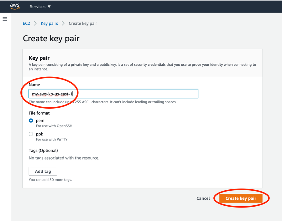

Step 3 ERM keypair

Live demonstration

HDFS Under the Hood: Read Algorithm

HDFS File System Demo

Ingest data from relational database to HDFS

Kafka Introduction

Kafka is a popular framework for building "event-based", "always-on" applications. Kafka is a distributed system consisting of servers and clients that communicate via a high-performance TCP network protocol. It can be deployed on bare-metal hardware, virtual machines, and containers in on-premise as well as cloud environments.

Kafka combines three key capabilities so you can implement your use cases for event streaming end-to-end with a single battle-tested solution:

1. To publish (write) and subscribe to (read) streams of events, including continuous import/export of your data from other systems.

2. To store streams of events durably and reliably for as long as you want.

3. To process streams of events as they occur or retrospectively.

And all this functionality is provided in a distributed, highly scalable, elastic, fault-tolerant, and secure manner. You can choose between self-managing your Kafka environments and using fully managed services offered by a variety of vendors. In the demo later on this page, we will be using Amazon's "Managed Streaming For Kafka (MSK)" service

Kafka Use Cases

Below are some examples of Kafka use cases.

1. Banking/Finance: Process payments and financial transactions in real-time

2. Automobiles/Logistics: Track and monitor vehicles, and shipments in real-time

3. IoT: Continuously capture and analyze sensor data from IoT devices or other equipment in public places or manufacturing units

4. Retail/Travel/Mobile Apps Collect and immediately react to customer interactions and orders

5. Healthcare/Insurance: Monitor patients in hospital care to ensure a timely treatment in emergencies.

6. Data Lake/Microservices: Serve as the foundation for data platforms, event-driven architectures, and microservices.

Kafka Concepts and Terminologies

Servers/Brokers:

• Kafka is run as a cluster of one or more servers that can span multiple data centers or cloud regions. Some of these servers form the storage layer, called the brokers.

• Kafka provides built-in scalability and fault tolerance capabilities. If any of the servers fail in the cluster, the other servers will take over their work to ensure continuous operations without any data loss.

Clients:

• Kafka Clients allows writing distributed applications and microservices that read, write, and process streams of events in parallel, at scale

• Kafka ships with some such clients included, which are augmented by dozens of clients provided by the Kafka community:

• Clients are available for Java and Scala including the higher-level Kafka Streams library, for Go, Python, C/C++, and many other programming languages as well as REST APIs.

Kafka APIs

Kafka includes five core apis:

1. Producer API: Allows applications to send streams of data to topics in the Kafka cluster.

2. Consumer API: Allows applications to read streams of data from topics in the Kafka cluster.

3. Streams API: Allows transforming streams of data from input topics to output topics.

4. Connect API: Allows implementing connectors that continually pull from some source system or application into Kafka or push from Kafka into some sink system or application.

5. Admin API: Allows managing and inspecting topics, brokers, and other Kafka object

Kafka Broker

A Kafka server, a Kafka broker and a Kafka node all refer to the same concept and are synonyms. A Kafka broker receives messages from producers and stores them on disk keyed by unique offset. A Kafka broker allows consumers to fetch messages by topic, partition and offset. Kafka brokers can create a Kafka cluster by sharing information between each other directly or indirectly using Zookeeper. A Broker is a Kafka server that runs in a Kafka Cluster. Kafka Brokers form a cluster. The Kafka Cluster consists of many Kafka Brokers on many servers.

Kafka Topic

A Topic is a category/feed name to which records are stored and published. As said before, all Kafka records are organized into topics. Producer applications write data to topics and consumer applications read from topics.

When to use?

• Sqoop: When you need to copy data from relational sources into Hadoop

• Kafka: When you need to ingest real-time

Examples of other ingestion tools

• Google PubSub

  • Pub/Sub offers durable message storage and real-time message delivery at scale.

• Apache Nifi

  • Automates the flow of data between software systems

• Amazon Kinesis

  • Ingest, buffer, and process streaming data in real-time

• Amazon Kinesis Firehose

  • Loads streaming data into data lakes, data stores, and analytics service

Map Reduce Word Count Walkthrough

Apache Pig Demonstration and Example

• Pig's infrastructure layer consists of a compiler that produces sequences of Map-Reduce programs, for which large-scale parallel implementations already exist (e.g., the Hadoop subproject).

• Pig's language layer currently consists of a textual language called Pig Latin, which has the following key properties:

  1. Ease of programming: It is trivial to achieve parallel execution of simple, "embarrassingly parallel" data analysis tasks. Complex tasks comprised of multiple interrelated data transformations are explicitly encoded as data flow sequences, making them easy to write, understand, and maintain.

  2. Optimization opportunities: The way in which tasks are encoded permits the system to optimize their execution automatically, allowing the user to focus on semantics rather than efficiency.

  3. Extensibility: Users can create their own functions to do special-purpose processing.

  https://youtu.be/V3RcOma9_EU

Creating Hive Table using HQL (Hive Query Language)

Loading Data into Hive Tables

Hive Internal and External Tables

Hive Partitioning

Hive organizes tables into partitions. It is a way of dividing a table into related parts based on the values of partitioned columns such as date, city, and department. Using partition, it is easy to query a portion of the data.

The idea here is that when you run a specific query such as "SELECT * FROM TABLE_NAME WHERE YEAR = 2020", and assuming you have 100 years worth of data in the table, hive does not have to read all the data. It can go to the partition (a subdirectory on HDFS under the main or root directory of the HDFS hive is pointing to) of the corresponding year.

Partitioning is a great way to optimize your queries and manage your data.

Select the partitioning column carefully. You want to select a column that leads to a category or groups a large chunk of data. Here are some good and bad examples of partitioning columns.

BAD Partition Column examples

• Primary Key column of some data set (Bad because you will end up creating one partition for each record of the table, leading to millions of directories)

• EmailID column of a dataset where each record is identified by email ID

• SSN column

GOOD Partition Column examples

• Partition the data based on Country where you have data from hundreds of countries

• Partition the data based on the State where you have data from multiple states within a country

• Partition the data based on Year where you have data from many different years

Why Partitioning is important?

• Partitioning the table makes the queries more efficient. When a query is executed with a partition column specified in the "WHERE clause, Hive can skip reading the complete table directory and all the corresponding partitions. Instead, it only reads the specific partition whose value is described in the SQL statement

• Partitioning also helps you organize your table data in a better way

• Typical example of partitioning columns are "YEAR", "MONTH", "DAY", "STATE", "CITY", "COUNTRY" etc.

Summary

Apache Static vs Dynamic Partitioning

• In Static partitioning, you need to know the value of the partitioning column at the time of the data load. Data also needs to be pre-segregated based on the corresponding partition key values

• In Dynamic partitioning, Hive runs a query to read the value of the partitioning column from each record in the data set and split them to the correct partition automatically. No need to be aware of the values of the partition column and no need to have pre-segregated data.

Read and explore more here: https://cwiki.apache.org/confluence/display/Hive/LanguageManual+DML#LanguageManualDML-DynamicPartitionInserts

Apache Spark Under The Hood

Resilient Distributed Data Sets

Spark RDD

• Fundamental data structure of Apache Spark

• It is an immutable (Read Only) distributed collection of objects

• Each dataset in RDD is divided into logical partitions

• RDDs may be computed on different nodes of the spark or Hadoop cluster

• Two ways to create RDDs

  • Parallelizing an existing collection in your driver program,

  • Referencing a dataset in an external storage system, such as a shared file system, such as HDFS

• Spark leverages the concept of RDD to achieve faster and efficient MapReduce operations

Operations on RDD

1. Transformations

2. Actions

RDD Lineage

• Resilient Distributed Dataset (RDD) Lineage is a graph of all the parent RDD of a RDD. Spark tries to keep the data in-memory (RAM) and due to failure, there is a risk of losing that data.

• In case some Dataset is lost, it is possible to use RDD Lineage to recreate the lost Dataset.

• Therefore RDD Lineage provides a solution for better performance of Spark as well as it helps in building a resilient system.

• It is built as a result of applying transformations to the RDD and creates a logical execution plan

• Logical Execution Plan starts with the earliest RDDs (those with no dependencies on other RDDs or reference cached data) and ends with the RDD that produces the result of the action that has been called to execute.

• See the following image for an example of Spark Lineage

RDD Lineage

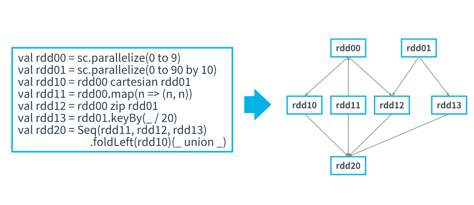
RDD Lineage

Image Description

• A Spark application code is represented with Directed Acyclic Graph known as (DAG)

• As we know, RDDs are read-only. When transformation functions are applied on RDD, they create a new RDD

• The picture above shows, how to code on the left side is interpreted by Spark when the logical execution plan is created

• RDD Lineage plays a crucial role in achieving the "Resiliency" property of RDD

• When a failure happens in Spark Cluster, with the help of RDD lineage, lost partitions can be quickly recomputed

• In this example, say the node on which RDD13 was hosted is a failure, based on the RDD lineage, it's known that RDD13 was really created from RDD01. So RDD13 can be recomputed on a live node

• Keep in mind that RDD lineage is only the metadata about the flow of RDD. Lineage does not contain actual data

• RDDs are more efficient than MapReduce in terms of resilience and fault tolerance. This is because, in MapReduce, when a failure happens in an interactive job, the whole job needs to be restarted. While RDDs can recompute precisely the lost work (with help of RDD lineage) and recover much faster

Getting started in Spark

Understanding the code of the Word Count Demo

DEMO: Spark Demo: Spark Submit, Performance, & Navigating Spark

Download sample data

wget https://video.udacity-data.com/topher/2020/November/5fabec84_game-reviews.tsv/game-reviews.tsv.gz

Data has the following schema. Please maintain the sequence of the column names while creating Hive table.

marketplace,    
customer_id, 
review_id,    
product_id,    
product_parent,    
product_title,    
product_category, 
star_rating,
helpful_votes,
total_votes,
vine,
verified_purchase,
review_headline,
review_body,
review_date

Data Format: TSV

Data is compressed. Hive automatically detects compressed tsv data. No need to unzip it and then load. You can load the file directly in hive table

Load data on HDFS

hdfs dfs -mkdir /game_reviews
hdfs dfs -put game-reviews.tsv.gz /game_reviews/

PySpark code for reference. Find top 10 users with highest number of review submissions.

Package the following code in sparkDemo.py file

from pyspark.sql import SparkSession

spark = SparkSession \
    .builder \
    .config("spark.some.config.option", "some-value") \
    .getOrCreate()

df = spark.read.option("sep", "\t").option("header",True).csv("/game_reviews/")

#df.show()

df.createOrReplaceTempView("game_reviews")

# Retrive the user ID with highest number of review submitions

responseDF = spark.sql("SELECT customer_id, count(*) num_reviews from game_reviews group by customer_id order by num_reviews desc limit 10");

responseDF.show()

Submitting Spark jobs to cluster using Spark Submit Command

spark-submit --master yarn --name SparkDemo sparkDemo.py

• You can pass many more parameters to Spark-submit command and control the infrastructure

• Generally you provide driver and executor memory, number of executors and and executor cores

• Learn more about submitting Spark applications to cluster

Spark Cluster Managers

Spark supports below cluster managers:

• Standalone – a simple cluster manager included with Spark that makes it easy to set up a cluster.

• Apache Mesos – Mesons is a Cluster manager that can also run Hadoop MapReduce and Spark applications.

• Hadoop YARN – the resource manager in Hadoop 2. This is mostly used, cluster manager.

• Kubernetes – an open-source system for automating deployment, scaling, and management of containerized applications.

• local – which is not really a cluster manager but still I wanted to mention as we use “local” for master() in order to run Spark on your laptop/computer.

YARN: Resource management in Hadoop Cluster

SQL abd NoSQL Comparison

Introduction to DynamoDB

DynamoDB Deep Dive

Demo Capacity Modes and Auto Scaling

#!/bin/sh
aws dynamodb create-table --table-name sampledata \
--attribute-definitions AttributeName=PK,AttributeType=S AttributeName=GSI_1_PK,AttributeType=S \
--key-schema AttributeName=PK,KeyType=HASH \
--provisioned-throughput ReadCapacityUnits=5,WriteCapacityUnits=5 \
--tags Key=workshop-design-patterns,Value=targeted-for-cleanup \
--global-secondary-indexes "IndexName=GSI_1,\
KeySchema=[{AttributeName=GSI_1_PK,KeyType=HASH}],\
Projection={ProjectionType=INCLUDE,NonKeyAttributes=['bytessent']},\
ProvisionedThroughput={ReadCapacityUnits=5,WriteCapacityUnits=5}"

FIleName: lab_config.py

boto_args = {'service_name': 'dynamodb'}

FileName: load_ddb_sampledata.py

from __future__ import print_function # Python 2/3 compatibility
import boto3
import time
import csv
import sys
from lab_config import boto_args


def import_csv(tableName, fileName, attributesNameList, attributesTypeList):
    dynamodb = boto3.resource(**boto_args)
    dynamodb_table = dynamodb.Table(tableName)
    count = 0

    servererror = False
    time1 = time.time()
    with open(fileName, 'r', encoding="utf-8") as csvfile:
        myreader = csv.reader(csvfile, delimiter=',')
        for row in myreader:
            count += 1
            newitem = {}
            for colunm_number, colunm_name in enumerate(attributesNameList):
                newitem[colunm_name] = attributesTypeList[colunm_number](row[colunm_number])
            # Create primary keys
            newitem["PK"] = "request#{}".format(newitem['requestid'])
            newitem["GSI_1_PK"] = "host#{}".format(newitem['host'])

            if newitem['responsecode'] == 500:
                newitem['servererror'] = '5xx'

            item = dynamodb_table.put_item(Item=newitem)

            if count % 100 == 0:
                time2 = time.time() - time1
                print("row: %s in %s" % (count, time2))
                time1 = time.time()
    return count

if __name__ == "__main__":
    args = sys.argv[1:]
    tableName = args[0]
    fileName = args[1]

    attributesNameList = ['requestid','host','date','hourofday','timezone','method','url','responsecode','bytessent','useragent']
    attributesTypeList = [int,str,str,int,str,str,str,int,int,str]

    begin_time = time.time()
    count = import_csv(tableName, fileName, attributesNameList, attributesTypeList)

    # print summary
    print('RowCount: %s, Total seconds: %s' %(count, (time.time() - begin_time)))

Command to update the table

#!/bin/sh
aws dynamodb update-table --table-name sampledata \
--provisioned-throughput ReadCapacityUnits=100,WriteCapacityUnits=100

Demo Capacity Modes and Auto Scaling

Managing and Understanding DynamoDB Capacity Changes

Accessing DynamoDB

You can access DynamoDB (or any other AWS service) in 3 different ways.

1. Using AWS Console (Graphical User Interface)

2. Using AWS CLI (Command Line Interface)

3. Using Programming Language of your choice - AWS offers a series of SDK (Software Development Kits) in multiple popular programming languages. Supported languages are C++, .Net, Java, Go, Python, JavaScript, Node.js, Ruby

In real world, you will either use CLI or Programming Language to interact with DynamoDB. Let's see how can we do that

aws dynamodb create-table \
    --table-name Movies \
    --attribute-definitions \
        AttributeName=Actor,AttributeType=S \
        AttributeName=MovieTitle,AttributeType=S \
    --key-schema \
        AttributeName=Actor,KeyType=HASH \
        AttributeName=MovieTitle,KeyType=RANGE \
--provisioned-throughput \
        ReadCapacityUnits=10,WriteCapacityUnits=5
        

How to create, update DynamoDB Items using AWS CLI

3 Ways to retrieve data from DynamoDB

1. GetItem API - Retrieve specific Item when you know both Primary Key and Sort Key

2. Query API - Retrieve specific Item when you know Primary Key but do not know Sort Key

3. Scan API - Open ended search in "entire" table. Scan operation is expensive on large tables and should be avoided

aws dynamodb put-item \
--table-name Movies  \
--item \
    '{"Actor": {"S": "Brad Pitt"}, "MovieTitle": {"S": "A River Runs Through It"}, "StudioTitle": {"S": "Western Studios"}, "Awards": {"N": "2"}}'


aws dynamodb put-item \
--table-name Movies  \
--item \
    '{"Actor": {"S": "Brad Pitt"}, "MovieTitle": {"S": "Once Upon a Time in Hollywood"}, "StudioTitle": {"S": "NBJ Studios"}, "Awards": {"N": "1"}}'

aws dynamodb put-item \
    --table-name Movies \
    --item \
    '{"Actor": {"S": "Saoirse Ronan"}, "MovieTitle": {"S": "Little Women"}, "StudioTitle": {"S": "NewFlux Studios"}, "Awards": {"N": "3"} }'

aws dynamodb put-item \
--table-name Movies  \
--item \
    '{"Actor": {"S": "CYNTHIA ERIVO"}, "MovieTitle": {"S": "Harriet Tubman"}, "StudioTitle": {"S": "Century Studios"}, "Awards": {"N": "4"}}'

aws dynamodb put-item \
    --table-name Movies \
    --item \
    '{"Actor": {"S": "Feras Fayyad"}, "MovieTitle": {"S": "The Cave"}, "StudioTitle": {"S": "Bloom Studios"}, "Awards": {"N": "7"} }'
    

NOSQL Data Modeling

Other NoSQL Databases

DynamoDB is just one of many other popular and powerful NoSQL databases out there. We encourage you to explore other NoSQL database solutions as well.

Cassandra

• Open-source, distributed NoSQL database

• Originally developed internally at Facebook and was released as an open-source project in July 2008

• Cassandra delivers continuous availability (zero downtime), high performance, and linear scalability that modern applications require, while also offering operational simplicity and effortless replication across data centers and geographies.

• Explore more here

• Cassandra home page

HBase

• Open-source non-relational distributed database

• Modeled after Google's Bigtable and written in Java

• Developed as part of Apache Software Foundation's Apache Hadoop project and runs on top of HDFS

• Explore more here

MongoDB

• MongoDB is a general-purpose, document-based, distributed database

• Uses rich JSON format

• Offers powerful Query APIs

• Explore more here

• Wikipedia

CouchDB

• Open-source document-oriented NoSQL database, implemented in Erlang

• CouchDB uses multiple formats and protocols to store, transfer, and process its data,

• It uses JSON to store data, JavaScript as its query language using MapReduce, and HTTP for an API

• Explore more here

What is a Data Lake

As a Data Architect, you have full control over how exactly you store the data in the data lake. This is in contrast to RDBMS systems where the engine stores the data internally in a proprietary format. As a Data Architect, you will have to take into consideration multiple elements of a given data format such as type of storage format (row-oriented vs columnar oriented), size of the data, schema evolution capabilities, splitability, and compression. In this section, we will explore some of these elements. As a Data Architect, the design decision you make around selecting the data format is one of the most crucial ones with long-term impacts on cost, performance as well as maintenance overhead of the data lake storage.

Consideration 1: File Size

One major consideration is the general size of each file in your data lake. As we learned in lesson 2, HDFS stores data into 128 MB (default size in most environments ) chunks. Every file is represented by multiple blocks (also called "Objects", or "Chunks") in the Hadoop cluster. As we learned in lesson 2, these blocks reside on the data node. Each block is registered with a name node ("metadata"). Each metadata entry for each block residing in the name node consumes about 150 bytes. Too many small files in a data lake with a large volume of data will lead to a large number of files and hence the amount of metadata that the name node is holding will also increase.

Imagine this way: If you have a book of 500 pages, however, the "Table of Contents" of the book itself is 250 pages, the table of content becomes less useful and it will take you much longer to find out the exact page number for the lesson you wanna read.

To put this in perspective, 100 million files, each using a block, would use about 30 gigabytes of memory in the name node.

Hadoop ecosystem tools are not optimized for efficiently accessing small files since reading a large number of small files comes with high I/O overhead. So take away here is that using a small number of larger files will lead to better performance than a large number of small files. If you have a use case where you inherently get smaller files, oftentimes, companies run nightly or hourly jobs to consolidate smaller files into bigger files.

Consideration 2: Type of Storage (Row Oriented vs. Columnar Oriented)

There are multiple data formats such as CSV, TXT, Parquet, ORC which can be used to store data. These formats differ in how they actually store data. Data can be stored in 2 different ways.

1. Row Oriented Format

2. Column Oriented Format

Let's explore them one by one.

Row Oriented Format

• Traditional and very popular format where data is stored and retrieved one row at a time and hence could read unnecessary data if some of the data in a row are required.

• Example: if you have a table with 1000 columns, and when you only need to read only 10 columns, you will still need to read the entire row (of 1000 columns) and then filter out unnecessary data. Because of this, row-oriented data formats (such as CSV, TXT, AVRO, or relational databases) are NOT efficient in performing operations applicable to the entire datasets and hence aggregation in row-oriented is an expensive job or operations.

• Records in Row Oriented Datastores are easy to read and write. Often times relational databases are uses this mechanism for online transaction system.

• Typical compression mechanisms which provide less efficient result than what we achieve from column-oriented data stores.

Column Oriented Format

• Data is stored and retrieve in columns and hence it can only able to read only the relevant data if required.

• Example, if you have a table with 1000 columns, and when you only need to read only 10 columns, there is NO need to read the rest of the columns at all. This leads to huge performance enhancements.

• Many big data technology tools such as Parquet and NoSQL databases are optimized to deal with Column-oriented formats leading to efficient performance.

• Column-oriented data formats offer high compression rates due to little distinct or unique values in columns.

Consideration 3: Schema Evolution

The schema of the dataset refers to its structure or organization. In databases, we develop DDL statements such as "CREATE TABLE..." to define the table schema (table name, column names, data types, primary keys, foreign keys, etc. ). We retrieve the schema or the metadata of the individual data set using SQL statements such as "Describe Table". In its simplest form, column headers of a CSV file can be considered schema.

As a Data Architect, you need to assess if the schema of your data set is anticipated will be changed or evolved over time. You need to determine how will your file format deal with newly added or deleted columns? Often times in IoT use cases, as device manufacturers upgrade the software and hardware over time, the device can send out data with a modified schema structure.

When evaluating schema evolution specifically, some of the key questions to ask of any data format are following:

1. Does the data format support schema evolution?

2. What is the impact on the existing data set if the new data set is received with an updated schema?

3. How easy or hard is it to update the schema (such as adding, removing, renaming, restructuring, or changing the data type of a field)

4. Does your data need to be human-readable?

5. What is the impact of schema evolution over the file size and processing speed?

6. How would you store different versions of the schema?

7. How different versions of the schema will integrate with each other for processing?

Consideration 4: Compression

Data compression reduces the amount of storage or transmission needed of a given set of data. With data compression, you can reduce the storage costs, and efficiently transmit the data over the network reducing resource utilization. As mentioned earlier, columnar data can achieve better compression rates than row-based data. It's more efficient to compress the data set by column since the data in the given column would be of the same type. For example, storing all "zip codes" together leads to more efficient compression rather than storing data of various types next to each other such as string, number, date, string, date. Compressed data would need to be decompressed at some point and decompression will incur additional compute costs. Generally, compression is recommended; however, you should always consider the impact on performance vs. reduced storage cost for your given use case.

Popular compression mechanisms used in Big Data are: "gzip", "bzip2", "lzo", and "snappy". Depending on the type of compression you can get a significant reduction in your data size (as high as 70 to 80%). You should also use compression formats that are "splittable". You will learn more about it in the next section.

Consideration 5: Splitability

As we learned in Lesson 3 (Ingestion, Storage and Processing), processing large amounts of data (terabytes to petabytes) requires breaking the processing job into multiple parts that execute independently (e.g MapReduce/Spark). The ability to break the data down into smaller blocks and processing these blocks in parallel is the key to efficient processing and speed. Choice of file format can critically affect the ease with which this parallelization can be implemented. For example, if each file in your dataset contains one massive XML structure or JSON record, the files will not be “splittable”, i.e. decomposable into smaller records that can be handled independently.

The general best practice is to always use a data format that offers splitability. Keep in mind that applying a compression mechanism sometimes makes a splittable data set into the unsplittable data set. For example, if you have a text file or csv file to process its content is splittable. However, if you compress the txt file with either "gzip", "bzip2" compression mechanisms, then the file is not splittable anymore reducing processing efficiency since the file can not be broken down into smaller blocks and processed in parallel.

Please refer to the table below to understand the various properties of various compression techniques.

Compression Format	Splittable?	Read/Write Speed	Compression Level
.gzip	No	Medium	Medium
.bzip2	Yes	Slow	High
.lzo	Yes, if indexed	Fast	Average
.snappy	No*	Fast	Average

*if Snappy compression is used with Parquet format, it's splittable. More on this in the next section

Data format

As a data architect, one of your jobs is to understand the use case, technical/business requirements, and then choose the correct data format to store data. In the last section, we learned what are some of the considerations for making this decision. In this section, we will dive deep into individual data formats, their advantage, and disadvantages. Popular formats are CSV, JSON, AVRO, PARQUET, and ORC. Among these Parquet is the most popular and defacto standard for data analytics. JSON is popular when it comes to streaming data, especially in IoT use cases.

• Row Oriented Data Formats: CSV, AVRO

• Column Oriented Data Formats: ORC, PARQUET

Further Learning (Links):

• AVRO Documentation

• Parquet Documentation

• ORC Documentation

• SON Information

CSV

A comma-separated values (CSV) file is a delimited text file that uses a comma to separate values. Oftentimes, instead of a comma, you can also have other characters as separators. CSV files represent the data in simple, human-readable plain text format. Each line contains 1 record and each record can have one or more fields. CSV format is not fully standardized. Oftentimes, instead of a comma, you can also have other characters as separators such as tabs or spaces or "|" "pipe" as a separator.

In its raw form, CSV files are splittable. However, please note that if you apply a nonsplittable compression mechanism (such as gZip) to compress CSV data, your file will become unsplittable. CSV files often have the first record showing the table headers or column names. Compared to XML, CSV files are compact, easy to read and parse. Unlike, JSON, CSV does not support complex data structures. CSV files also do not provide any support for indexing or column level data types.

An example of CSV file is below:

id, name, age, email
1, Rob, 76, [e-mail]
2, John, 43, [e-mail]
3, Bob, 23, [e-mail]
4, Su, 67, [e-mail]

JSON

JSON (JavaScript Object Notation), ) is a very common, popular data format with a diverse range of applications. It's a defacto standard for many of the REST APIs to exchange data. JSON data is human-readable and represents the data in "key" - "value" format. JSON is often used as a low-overhead replacement for XML in modern systems. JSON allows hierarchical and nested structures. Many NoSQL databases such as MongoDB, DynamoDB, Couchbase allows you to store and query JSON documents. Most modern Big Data tools support JSON format.

JSON data can also be represented in performance-optimized and compressed formats such as Parquet and Avro. JSON is also a pretty standard way to streaming IoT data. Unlike CSV format, JSON structure is well defined and standardized. JSON supports basic data types such as Number, String, Boolean, Array, and Null. Many libraries and packages work with all popular programming languages to read, parse and write JSON data. Examples of such libraries are: "JSON.simple" , "GSON", "Jackson" and "JSONP".

Below is an example of JSON data:

{
  "firstName": "Alex",
  "lastName": "West",
  "isAlive": true,
  "age": 35,
   "email": "[e-mail]"
  "address": {
    "streetAddress": "6300 Hollywood Boulevard",
    "city": "Los Angeles",
    "state": "CA",
    "postalCode": "90028"
  },
  "phoneNumbers": [
    {
      "type": "home",
      "number": "212 555-1234"
    },
    {
      "type": "office",
      "number": "646 555-4567"
    }
  ],
  "children": [],
  "spouse": null
}

Parquet

"Apache Parquet is a columnar storage format available to any project in the Hadoop ecosystem, regardless of the choice of data processing framework, data model or programming language"(Apache Parquet. https://parquet.apache.org/). Apache Parquet is a free and open-source format popular in processing Big Data workloads. It is similar to the other columnar-storage file formats available in Hadoop namely RCFile and ORC. Popular Big Data processing frameworks such as Apache Hive, Apache Drill, Apache Impala, Apache Crunch, Apache Pig, Cascading, Presto, and Apache Spark support Parquet format.

Parquet uses snappy as the default data compression mechanism and provides column level compression to reduce storage space. Parquet files are not human-readable. Parquet allows queries to fetch/read specific column values that need not read the entire row data which significantly improves performance. Parquet provides better compression and encoding with improved read performance at the cost of slower writes (following WORM paradigm - "Write Once Read Many").

Apache Parquet supports "limited" schema evolution. Parquet files store the schema information along with the files themselves. It also provides the ability to add new columns and merge schemas that don't conflict. Parquet also supports "Predicate Pushdown" - allowing it to skip reading blocks of data, further improving query performance. Due to these properties, Parquet is the most popular and defacto data standard when it comes to building large scale "Data Lakes" on Cloud or using HDFS.

ORC (Optimized Row Columnar)

The Optimized Row Columnar (ORC) file format provides a highly efficient way to store data in the columnar structure. Using ORC files improves read/write performance. An ORC file contains groups of row data called stripes, along with auxiliary information in a file footer.

Compression parameters, as well as the size of the compressed footer, are stored at the end of the file. Stripe size defaults to 250 MB. Large stripe sizes can be used for large, efficient reads from HDFS. The file footer contains items such as 1)list of stripes in the file, 2)the number of rows per stripe, and 3)each column's data type; also included is aggregates such as count, min, max, and sum. These stripes are the data building blocks of ORC format and independent of each other, which means queries can skip to the stripe that is needed for any given query, improving performance.

ORC includes support for ACID transactions, built-in indexes (implemented via stripes) allows skipping to the right row with indexes including minimum, maximum, and bloom filters for each column. ORC supports all of Hive's types including the compound types: structs, lists, maps, and unions.

AVRO

Unlike Parquet, ORC, and RCFile formats, AVRO is a row-oriented data format. AVRO is open source and allows splitting. AVRO also supports schema evolution. The schema is stored alongside the Avro data so that files may be processed later by any program. If the program reading the data is expecting a different schema than what is currently stored, this can be easily resolved, since both schemas are present. AVRO uses JSON for defining data types and serializes data in a compact binary format. This facilitates implementation in languages that already have JSON libraries.

Following is an example of an AVRO schema. Schemas are composed of primitive types (null, boolean, int, long, float, double, bytes, and string) and complex types (record, enum, array, map, union, and fixed).

{
   "namespace": "example.avro",
   "type": "record",
   "name": "Product",
   "fields": [
      {"name": "name", "type": "string"},
      {"name": "product_number",  "type": ["null", "int"]},
      {"name": "product_color", "type": ["null", "string"]}
   ] 
 }

electing the right data format for your organization's Data Lake is a crucial decision you will make as an architect which will have long-term impact on the size, scale, and performance of the system. Start by looking into various considerations (size, storage type - row vs column-oriented, schema evolution, compression, splittability). The data formats we discussed here is summarized in the table below:

	PARQUET	AVRO	ORC
Schema Evolution	Good	Best	Better
Compression	Better	Good	Best
Splitability	Good	Good	Best
Row vs. Column Oriented	Column	Row	Column
Read/Write Speed	Read	Write	Read

Data Lake/Big Data Formats

In this exercise, you will develop a series of Hive Query statements to convert a data set from CSV to Parquet format.

Data Formats

Complete the following tasks to convert CSV dataset into Parquet dataset using Hive

CREATE DATABASE IF NOT EXISTS NY_COLLISION;

set hive.cli.print.header=true;

CREATE EXTERNAL TABLE IF NOT EXISTS NY_COLLISION.CRASH_EXT(
    COLLISION_ID string,
    ACCIDENT_DATE string,
    ACCIDENT_TIME string,
    BOROUGH string,
    ZIPCODE integer,
    LATITUDE double,
    LONGITUDE double,
    LATLONG string,
    ON_STREET_NAME string,
    CROSS_STREET_NAME string,
    OFF_STREET_NAME string,
    NUMBER_OF_PERSONS_INJURED string,
    NUMBER_OF_PERSONS_KILLED string,
    NUMBER_OF_PEDESTRIANS_INJURED string,
    NUMBER_OF_PEDESTRIANS_KILLED string,
    NUMBER_OF_CYCLIST_INJURED string,
    NUMBER_OF_CYCLIST_KILLED string,
    NUMBER_OF_MOTORIST_INJURED string,
    NUMBER_OF_MOTORIST_KILLED string,
    CONTRIBUTING_FACTOR_VEHICLE_1 string,
    CONTRIBUTING_FACTOR_VEHICLE_2 string,
    CONTRIBUTING_FACTOR_VEHICLE_3 string,
    CONTRIBUTING_FACTOR_VEHICLE_4 string,
    CONTRIBUTING_FACTOR_VEHICLE_5 string,
    VEHICLE_TYPE_CODE_1 string,
    VEHICLE_TYPE_CODE_2 string,
    VEHICLE_TYPE_CODE_3 string,
    VEHICLE_TYPE_CODE_4 string,
    VEHICLE_TYPE_CODE_5 string)
    ROW FORMAT DELIMITED
    FIELDS TERMINATED BY ','
    LOCATION '/user/crash_ext';

LOAD DATA LOCAL INPATH 'sample-data-l2-e1.csv' OVERWRITE INTO TABLE NY_COLLISION.CRASH;

CREATE TABLE NY_COLLISION.CRASH_parquet STORED AS PARQUET LOCATION '/user/crash_parquet' AS SELECT * FROM NY_COLLISION.CRASH_EXT;

SELECT * FROM NY_COLLISION.CRASH_EXT LIMIT 10;
SELECT * FROM NY_COLLISION.CRASH_parquet LIMIT 10;

Elements of Data Lake

ntroduction to Data Lake Design Patterns

• Incremental processing on object storage is hard

• Updating one record requires rewriting the whole file!

• Individual record updates are very inefficient and lead to huge IO overhead

• Need Database like functionalists in Data Lake Object Storage

As data is written for the first time, or updated in real-time, for example from a SQL database, a data lake must handle the complete transaction from beginning to end, otherwise, data could be out of sync or inconsistent. Incremental processing can handle updates and deletes.

Apache Hudi

Hudi Table Types

Hudi supports the following table types.

Copy On Write:

• Stores data using exclusively columnar file formats (e.g parquet). Updates simple version & rewrites the files by performing asynchronous merge during write.

Merge On Read

• Stores data using a combination of columnar (e.g parquet) + row-based (e.g Avro) file formats. Updates are logged to delta files & later compacted to produce new versions of columnar files synchronously or asynchronously.

Query Types in Hudi

Hudi supports the following query types

Snapshot Queries:

• Queries see the latest snapshot of the table as of a given commit or compaction action.

• In case of merge on reading table, it exposes near-real-time data(few mins) by merging the base and delta files of the latest file slice on-the-fly.

• For a copy on write table, it provides a drop-in replacement for existing parquet tables, while providing upsert/delete and other write side features.

Incremental Queries:

• Queries only see new data written to the table, since a given commit/compaction.

• This effectively provides change streams to enable incremental data pipelines.

Read Optimized Queries:

• Queries see the latest snapshot of the table as of a given commit/compaction action.

• Exposes only the base/columnar files in the latest file slices and guarantees the same columnar query performance compared to a non-Hudi columnar table.

Write operations by Hudi data source

UPSERT:

• Default operation where the input records are first tagged as inserts or updates by looking up the index.

• The records are ultimately written after heuristics are run to determine how best to pack them on storage to optimize for things like file sizing.

• This operation is recommended for use-cases like database change capture where the input almost certainly contains updates.

INSERT:

• Similar to upsert in terms of heuristics/file sizing but completely skips the index lookup step.

• Thus, it can be a lot faster than upserts for use-cases like log de-duplication (in conjunction with options to filter duplicates mentioned below).

• This is also suitable for use-cases where the table can tolerate duplicates, but just need the transactional writes/incremental pull/storage management capabilities of Hudi.

BULK_INSERT:

• Both upsert and insert operations keep input records in memory to speed up storage heuristics computations faster (among other things) and thus can be cumbersome for initial loading/bootstrapping a Hudi table at first. Bulk insert provides the same semantics as insert while implementing a sort-based data writing algorithm, which can scale very well for several hundred TBs of initial load. However, this just does a best-effort job at sizing files vs guaranteeing file sizes as inserts/upserts do.

Explore more here:

• https://hudi.apache.org/docs/concepts.html

• https://hudi.apache.org/docs/writing_data.html

Apache Hudi is a tool to ingest & manage the storage of large analytical datasets over DFS (HDFS or cloud stores). It brings stream processing to big data, providing fresh data while being an order of magnitude efficient over traditional batch processing.

• Developed by Uber, powers their petabyte-scale data lake

• Became top-level Apache Project

Hudi Features

• Upsert support with fast, pluggable indexing

• Snapshot isolation between writer & queries

• Manages file sizes, layout using statistics

• Timeline metadata to track lineage

• Savepoints for data recovery

• Async compaction of row & columnar data

Hudi Data set

• Index - Map rows to individual files

• Timeline metadata - tracks changes

• Data file - actual files. Hudi leverages Parquet data format

• Hudi data set can be queried with Spark, Hive, Presto

Other similar & related systems

• Hive Transactions

• Databricks Delta Lake

• Apache Kudi

Resources and Links

• Explore Hudi more here

• Dive deep on Hudi concepts

• Explore Delta lake more here

GitHub - mattssll/udacity_data_architect: nanodegree_udacity_data_architectGitHub

Data Governance Is Important

Enterprise Conceptual Data Model - Example

Enterprise Logical Data Model

Types of Metadata

Part 3 - Ingestion and Curation

All the different metadata types are integrated and loaded into a Metadata Management System that can be easily accessed by anyone in the company. Some key uses of the Metadata Management System:

• Anyone in the company can search the metadata system to identify the location of data and reports they are looking for.

• All aspects of data like rules, definitions, lifecycle, lineage, ownership, quality, and usage are documented. This, in essence, provides a 360-degree view of data.

• Links business to technology by providing the ability to trace a business process to data entities and elements and the systems and tables where the data resides.

To achieve the different capabilities and functionality of a metadata management system, you can either buy a vendor product or build your own custom technology solution. The technology solution for Metadata Management System has the following basic components:

• User interface is used by business, technical and governance teams to create, curate, govern, and search for metadata.

• Central repository, where all the metadata is stored.

• Connectors enables automated metadata ingestion from different documents, databases, reporting tools, data modeling tools, ETL tools, and applications.

• Processing engine receives and processes the requests from the user interface, retrieves the necessary metadata from the repository, and loads the data retrieved by the connectors.

Steps involved in creating a Metadata Management System:

• Design an Enterprise Data Catalog based on the Enterprise Logical Data Model. This is done by identifying any existing business metadata, mapping each entity to all the systems where it resides, mapping attributes to tables and columns in different systems, and locating any existing technical metadata for the systems identified.

• Build an ingestion process to automatically parse and retrieve metadata from different sources and load it into the Metadata Management System.

• Curate the metadata in the user interface of the Metadata Management System to fill in the missing pieces that don't exist in the systems.

Different people involved in a Metadata Management System have different roles and responsibilities. Business subject matter experts create business metadata. Technical developers and architects create technical and operational metadata and create automated processes to ingest existing metadata into the Metadata Management System. Data Stewards in the governance teams review and approve the metadata created by different people to ensure metadata is consistent and follows the standards.

New terms

• Metadata Management System enables the consolidation, storage, and exploration of metadata.

• ETL abbreviation for Extraction, Transformation, and Load. Gathers data from multiple source systems, consolidates, and loads into a destination system.

Further reading

You can review this article to understand the different vendor products available for metadata management.NEXT

Data Quality Management

Data Profiling

ata profiling is a process where you analyze the data from different sources and summarize information about data. Data profiling should be one of the first steps in a data project. Data profiling is used to understand the data, discover business rules, and identify data quality issues. Some of the most commonly used data profiling techniques:

First, you perform some basic profiling to analyze the data in a table and each of the columns using different techniques:

• Table Profiling is a process where you perform some high-level profiling of the data in a table. More specifically:

1. Reviewing the number of records in a table gives you an idea of how big the dataset is.

2. Reviewing some sample records, say 10-20 rows helps you understand the data,

• Column Profiling is a process where you analyze data in each column of a table. More specifically:

1. Number of unique values helps you identify the columns that should have a finite set of values, for example, product category, sales district, gender. This helps with query optimization.

2. Number of null and blank values can help determine data quality issues like incomplete data from a source.

3. Maximum and minimum values help determine the range of the dataset and identify any potential outliers.

4. Data type and length inference help during the creation of the data model. It also helps to identify issues like the revenue column having a text value.

Part 2 - Data Value Profiling

After you complete basic profiling on data, you perform an in-depth analysis of data values. As a result of this analysis, you identify data outliers which are data points that fall outside of the expected list of values. There are different types of outliers:

• You examine the data values in a column to identify outliers. For example, some of the records are assigned to the ‘Unknown’ sales region.

• You look into patterns in the data to identify outliers. For example, some phone numbers in a column do not have an area code.

• You look into the distribution of data in a column to identify abnormal and potentially erroneous values. For example, some order records have a negative unit price.

You also analyze the data to identify the data domain which is the subject area of the data. For example, Product Code, Email Address, Social Security Number,

New terms

• Table Profiling: Process where you perform some high-level profiling of the data in a table

• Column Profiling: Process where you analyze data in each column of a table

• Data Outliers: Data points that fall outside of the expected list of values

• Data Domain: is the subject area of the data

Further reading

To understand the vendor tools available in the market for data profiling, you can read this articleNEXT